13 - Integrated Design Analysis

The Sigrity™ technology-driven environment of OrCAD X Presto offers robust high-speed analysis and checking through the Analysis Workflow panel. You can access Impedance and Coupling workflows by selecting OrCAD X Professional or OrCAD X Professional licenses. These intuitive workflows are designed to identify impedance mismatches in routed signals and excessive signal coupling without needing any models. Early detection of such issues allows design engineers to address and resolve them quickly, enhancing productivity and decreasing the time to market.

You can run these guided workflows, which include steps for initiating, executing, and reviewing the results of various analyses through the Analysis Workflows panel, accessible from View – Panels – Analysis Workflows. To run these workflows, set the SIGRITY_EDA_DIR to the directory of a Sigrity™ installation for the release 2024.1.

Performing Impedance Analysis

The impedance presented here is the characteristic impedance of a transmission line. At the frequencies of interest for most PCBs, this is Z_0 = sqrt(L/C) which does not depend on frequency. The L and C values are computed from the 2D cross-sectional geometry of the trace and reference. At lower frequencies, where the characteristic impedance does depend on frequency, matching impedances is usually not a concern because reflections will usually be minimal.

1. Choose View – Panels – Analysis Workflows.
2. Choose Impedance Workflow.
3. Choose either Net Based or Directed Group from Analysis Modes. Net Based is chosen by default.
4. Select nets or specify directed groups based on the analysis mode.
5. To include coplanar data in the simulation results, click Analysis Options and select Detect and model the coplanar traces.
6. Click Start Analysis.
   Progress of analysis is shown in the Analysis section of the Analysis Workflows window.
   When analysis is complete, a green check will appear for the Start Analysis task. If a previous analysis is stored, a prompt appears for overwriting the old analysis.
7. Click Save Analysis Results to save the results. Specify a name and location for the results file.
   The extension for the result file is .impida for impedance analysis.
8. Specify View Modes. Choose:
   • Net Based to view results for all segments of selected nets. Available for all analysis results.
   • Directed Group to view results for segments defined in selected directed groups. Available only if analysis results contain directed group data.
   • Single Ended to view single-ended analysis results for both single-ended and differential pair nets.
   • Diff Pair to view differential pair analysis results for differential pair nets and single-ended results for single-ended nets.
     Differential analysis results are reflected for coupled segments of differential pairs.

Impedance Vision

Clicking Impedance Vision displays color-coded impedance segments in the canvas.

The color coding is based on the segment or sub-segment impedance value as mapped into the im pedance gradient, which is the continuous transition of colors from the minimum to maximum range of impedance values obtained by analysis. Any nets part of the analysis results which have segments not associated with impedance analysis data will be displayed in the default color based on layer/net color assignments. Any nets which are not part of the analysis are dimmed in the default color.

The Single Ended view mode setting displays all Singled Ended impedance result for the selected nets; both single ended nets and differential pair nets of the results use single ended impedance data to color segments and for data tips.

The Diffpair view mode setting displays Single Ended impedance data for all single ended nets and all Diffpair impedance data for all differential pair nets.

Impedance Table

Summary Table lists summary impedance results for each net selected for analysis. Detailed Table lists the impedance results for each segment on the net selected in Summary Table.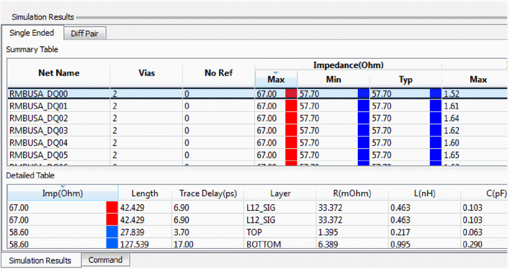


To sort data in the table, click any column header.

Select rows in the Detailed Table section to zoom/center the canvas on the impedance variance for investigation.

If view mode is Single Ended, a Single Ended tab appears at the top of the summary table and all net results appear in the summary table.

If view mode is Diffpair, both the Single Ended and Diffpair tabs appear at the top of the summary table. Select the Single Ended tab to view single ended nets or select the Diffpair tab to view differential pair nets.

Performing Coupling Analysis

Coupling is not computed at a single frequency. Since PCB traces carry bit patterns that are made of pulses containing many frequencies, the coupling coefficient result takes into account a rise time in picoseconds. The maximum frequency relevant to the trace is inversely proportional to rise time parameter.

1. Choose View – Panels – Analysis Workflows.
2. Choose Coupling Workflow.
3. Choose either Net Based or Directed Group from Analysis Modes. Net Based is chosen by default.
4. Select nets or specify directed groups based on the analysis mode.
5. Click Analysis Options.
   The Coupling Analysis Parameters dialog appears.
   Specify the following parameters:
   • Detect and model the coplanar traces: Choose to include coplanar data in the simulation results.
   • Coupling: Specify the minimum net level coupling coefficient threshold in percentage. The default value is 2%.
   • Rise Time: Specify the rise time for minimum coupled length in ps (picoseconds). The default is 50ps.
   • GeoWindow: Set a geometry window value in design units for aggressor inclusion for the selected victim nets. All net segments within the specified distance from the selected net across layers will be considered as aggressors. This is optional for coupling analysis and allows for additional potential aggressors to be found based on the window.
6. Click Start Analysis.
   Progress of analysis is shown in the Analysis section of the Analysis Workflows window. When analysis is complete, a green check will appear for the Start Analysis task. If a previous analysis is stored, a prompt appears for overwriting the old analysis.
7. Click Save Analysis Results to save the results. Specify a name and location for the results file.
   The extension for the result file is .cplida for coupling analysis.
8. Specify View Modes. Choose:
   • Net Based to view results for all segments of selected nets. Available for all analysis results.
   • Directed Group to view results for segments defined in selected directed groups. Available only if analysis results contain directed group data.
   • Worst case to view the maximum coupling coefficient for all segments of selected nets.
   • Victim to view aggressor segments for a selected victim net.
9. Click Coupling Table or Coupling Vision to view results.

Coupling Vision

Clicking Coupling Vision displays color-coded coupling segments in the canvas.

The color coding is based on the segment or sub-segment coupling coefficient value as mapped into the coupling color gradient, which is the continuous transition of colors from the minimum to maximum range of coupling values obtained by analysis. Nets which are not part of the analysis are dimmed in the default color. Even for a net that is part of the analysis, segments not associated with the analysis will be displayed in the default color based on layer/net color assignments.

The Worst Case view mode setting highlights segments on victim nets. The color coding is based on the maximum coupling coefficient for any aggressor segment to that victim segment. Victim segments not having a coupling coefficient are displayed dimmed in the default color.

The Victim view mode setting highlights aggressor segments and sets the color to active victim net/ segment. The color coding is based on the coupling coefficient for each aggressor segment to the cross-probed net/segment. The victim net is displayed in the default color. Aggressor segments not having a coupling coefficient applied to the victim net/segment are displayed dimmed in the default color.

Coupling Table

In the Coupling Table, Worst Case and Victim modes differ in the way aggressors are color coded in the table.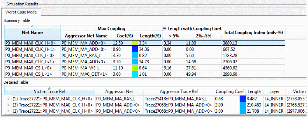

Summary Table lists summary coupling results for each net selected for analysis. Detailed Table lists the coupling results for each segment on the net selected in Summary Table.

Detailed Table provides a hierarchical view where each victim segment and all related aggressors are listed in one block of information as contiguous rows. Within the victim segment block, the aggressors are listed in the order of the highest coupling coefficient. If coupling coefficients are same, length is considered for ordering.

The first row in each block is the victim summary line and displays the total aggressor count for the block in the first column. If the block hierarchy is contracted, the aggressor with the highest coupling coefficient and longest length is displayed.

In the Worst Case mode, the coupling coefficient (Coupling Coef) column is color coded on the victim summary line and the maximum aggressor within the block. The coupling coefficient column for nonmaximum aggressors is colored gray.

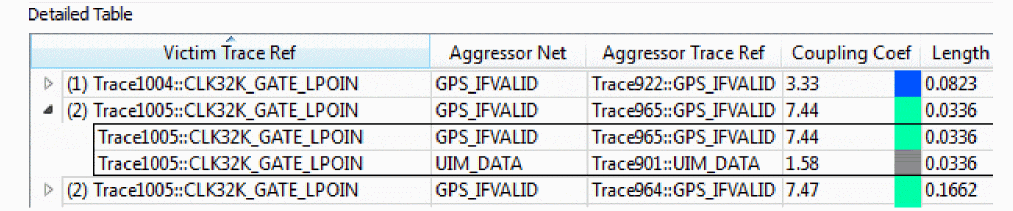
In the Victim mode, the coupling coefficient column is color coded for all aggressors but the victim summary line is gray. On the victim summary line, the victim segment column is color coded with the default color as it appears on the canvas.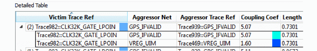

Selecting Nets

In a net-based analysis, every segment of the selected nets is simulated. Whereas, in a directed group, only net portions specified by a start component and one or more end components are simulated.

If analysis mode is set to Net Based, the Select Nets flow step is presented and marked with a cross to indicate that the step must be completed.

To select nets or modify a selection, do the following steps:

1. Click Select Nets to open the (X)Net Selection window.
   
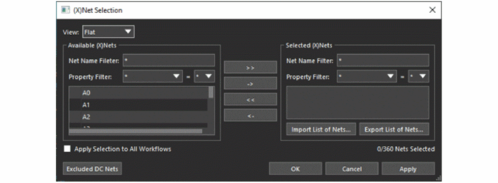
   The available nets are listed in the left pane and the selected nets in the right pane.
2. Select either Flat or Hierarchical from View.
   The Flat view lists all nets in the design in alphabetical order.
   The Hierarchical view lists the nets under defined hierarchy objects, such as differential pairs, net groups, bus, XNets, or nets.
3. You can add one or more nets directly from the canvas by clicking or windowing around nets. Click nets while pressing Ctl to remove them from selection.When done, right-click and choose Done or Clear All.
   Or, you can select available nets or XNets from the left pane and double-click to add to the selected list on the right. Similarly, select nets or XNets on the right plane and double-click to remove them from the selected list.
   Use the Available XNets/nets and Selected XNets/nets fields to filter out specific XNets/nets. You can also click the buttons in the middle to select nets. The >> button selects all available nets whereas << removes all selections. Voltage nets are excluded from the list of available nets. To see a list of the excluded nets, click Voltage Nets Excluded from List.
4. Click Apply to set the changes or click OK to set the changes and exit the dialog.
   The Select Nets step has a green check (  ) and you can proceed with the rest of the flow steps.

Specifying Directed Groups

In directed groups or component-based net selection, you can select an entire interface based on component connectivity rather than each net name.

Directed groups help prioritize issues; for example, issues found near the start point as compared to issues found near the end point. In addition, directed groups let you associate specific analysis results for a collection of nets as encountered along the same time-line as progressing from the start to the end point.

If analysis mode is set to Directed Group, the Select Directed Group flow step is presented and marked with a cross to indicate that the step must be completed.

To select, create, or modify directed groups or modify a selection; click Select Directed Group to open the Directed Group Selection dialog box.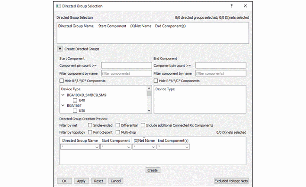

The top section, Directed Group Selection, lists the selected directed groups. A directed group is the portion of a net between a starting component and one or more ending components.

Use the expandable Create Directed Groups section to create directed groups.

To create a directed group, do the following steps:

1. Select a start component either on the canvas or from the list of components in the Start Component box or on the canvas.
   When you click a start component, all possible end components are visible while the other components are dimmed on canvas.
   The valid end components are listed under End Component.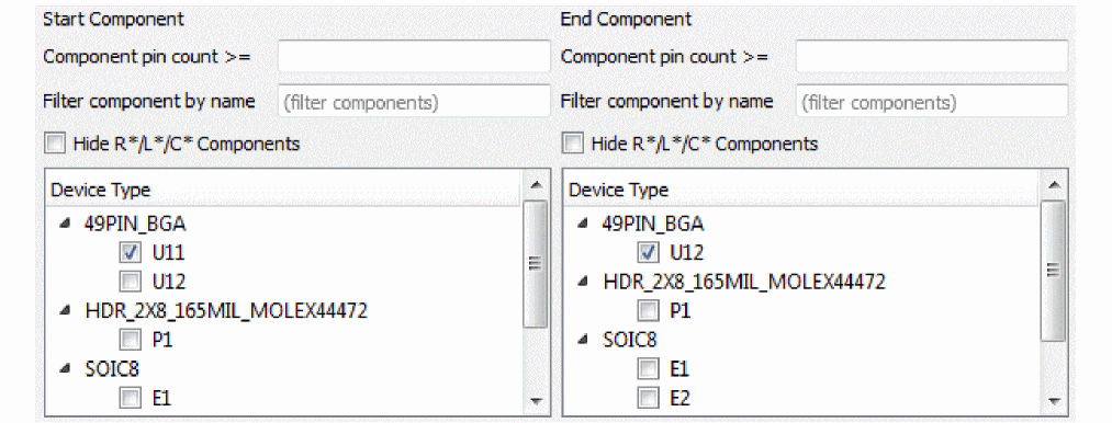
   
   Hide the passive components by selecting Hide R*/L*?/C* Components. You can also filter the list for ease of use.
2. Select one or more end components.
   A preview of the directed group is shown in the bottom section.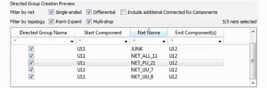
   
   
   All nets are selected by default. You can filter the list to display selected nets.
3. If needed, right-click in the preview area and choose any one of the options to select nets based on any filters.
   
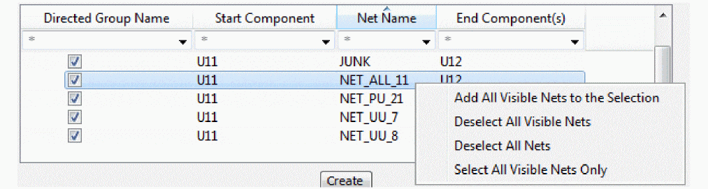
   The nets that are displayed based on the filter settings are the visible nets. In the example image, the filter is set to * to select all nets.
4. Click Create to create the directed group.
   The group is created and selected by default.

To select available directed groups or modify a section, do the following steps:

1. Select listed directed groups from the Directed Group Selection section. The selected groups are marked by a tick in the box on the left.
2. Click Apply to update the design or click OK to update the design and close the dialog box. The Select Directed Groups step has a green check and you can proceed with the rest of the flow steps